library(igraph)
library(ADAPTSNA)8 Subgraphs and Ego Graphs
Like all data-related research, there are scales of network data. By scales I mean that there are large-scale (macro) and small-scale (micro) network data. The focus of your analysis could be at the large scale, or what we call sociocentric scale, wherein you have multiple people and their connections. In these data, you might be working with population data (a complete network with every possible person and tie) or a sample of the population. At this level, your focus is on the entire group and how individuals relate to one another. On the other end of the scale, you might have individual-level network data, called egocentric networks. In these, the individual is the focal point of your data and you have their connections to and information about their alters. So far we have been dealing with sociocentric data and, largely, we will continue to do so. In the section on analysis we will cover egocentric network data, but, for now we will continue to work with full network data.
However, being mindful of the scale of your research is important. If you have complete network data (sociocentric) then you may want to zoom in on certain people or a certain person through a transformation tool called subgraph. There are two basic ways that you can think about this. You may be interested in a specific group of people and how they relate to each other. Therefore, you want to cut them from the sociocentric network and display a network based on how they relate to one another. This could be done by the name of people (i.e. specific nodes you want to see separate from the group). The second type of subgraph you may be interested in is an egocentric network of person to find out who they are connected to.
| LEARNING ELEMENTS - Data Discoveries |
|---|
|
In this chapter, we will cover the subgraph and ego graph capacities of transforming network data and explore instances where you might want to analyse these graph subsets. First, we start by bringing in the data and cleaning out the self loops. This new dataset is of some Grime musicians from Spotify. The nodes are the artists and the ties represent collaborations between the artists in 2008.
grime_edge_list <- load_data("GRIME_2008_Edge.csv", header = TRUE)

grime_08 <- graph_from_data_frame(d= grime_edge_list,
                                  directed = TRUE)
grime_08_clean <- delete_edges(grime_08,
E(grime_08)[which_loop(grime_08)])Specific Subgraphs
First, let’s assume you need a subgraph to see a specific set of people and how/whether they are connected. You may have a list of individual nodes that you are interested in and you want to see how they related to each other. You can do this by creating a vector with the names of those nodes, then use the subgraph function().
Why might you want to do this? There could be a highly prominent individual, or group of individuals in the network and you might want to see how these individuals are connected. Here, the individuals, Wiley, Jammer, Flowdan, and Ice Kid, are some of the older generation grime artists. In this network, taken from 2008, it might be interesting to see how/if these individuals are connected.
sub_people <- c('Wiley', 'Jammer', 'Flowdan', 'Ice Kid')

sub_net <- subgraph(grime_08_clean, sub_people)

par(mar = c(0,0,0,0))
plot(sub_net)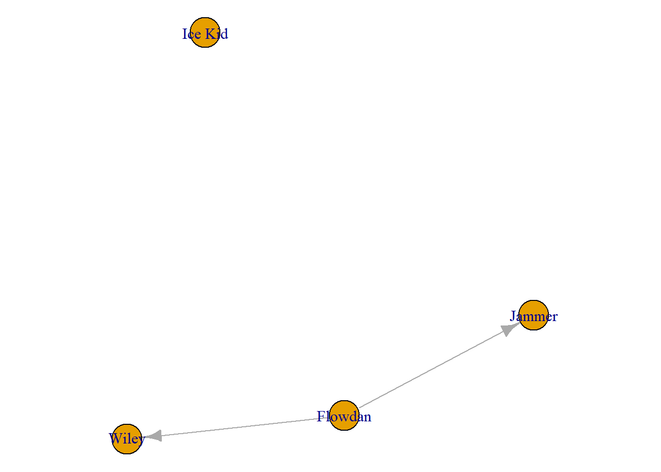
I encourage you to play around with this a little. Using the following code to identify the names of all the nodes in this network and then return to the chunk above. Copy over some of the names of the other artists to create different subgraphs of other artists to compare across different subgroups.
V(grime_08_clean)$name [1] "Asher D" "Dizzee Rascal" "Lethal Bizzle" "Scorcher"
[5] "Bless Beats" "Flowdan" "Tinchy Stryder" "Frisco"
[9] "Kano" "Treble Clef" "Shystie" "Blacks"
[13] "Badness" "Chronik" "Tempa T" "Newham Generals"
[17] "Skepta" "JME" "Chip" "BBK"
[21] "Virus Syndicate" "Ghetts" "Mercston" "Double S"
[25] "Griminal" "Ice Kid" "Nu Brand Flexxx" "Wretch 32"
[29] "Wiley" "Bossman Birdie" "The Streets" "Sway"
[33] "Tinie Tempah" "Giggs" "Jammer" "Roll Deep"
[37] "Devlin" "P Money " "Lauren Mason" "Milli Major" Another thing you could do with this tool is create a subgraph based on a certain characteristic the nodes have. For example, you might want to analyse the men in a network and how they are connected. To do so you would identify the names of the nodes who are male and pull out only the men from a network to have a male-only subgraph. Likewise, you could do a female-only network and compare the structure of the two networks.
Finally, one other way to can subset a network is by a set parameter you may have. For example, you may want to see a network of frequent collaborators (more than 1 collaboration). The following returns a vector with collaborators who work together more than once.
frequent_collabors <- E(grime_08_clean)[[collab_weight > 1]]

head(frequent_collabors)
+ 6/28 edges from 635c771 (vertex names):
[1] Scorcher ->Wiley Flowdan ->Wiley Tinchy Stryder->Wiley
[4] Blacks ->Jammer Badness ->Jammer Tempa T ->JammerYou can then turn this vector of edges into a igraph object to plot it. This demosntrates that you can create a specific subgraph not only from names of individuals but other characteristics or relational parameters.
frequent_collabors_graph <- induced_subgraph(
  grime_08_clean, vids =
    unique(c(ends(grime_08_clean, frequent_collabors)[, 1],
             ends(grime_08_clean, frequent_collabors)[, 2])))

plot(frequent_collabors_graph) 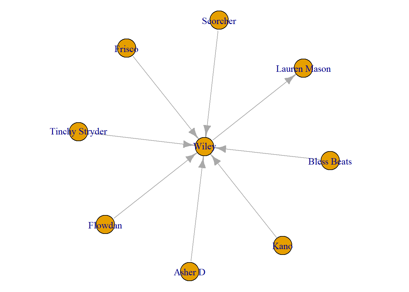
Ego Graphs
Next, you may want to see ego networks from those in your network. In other words, smaller networks showing only the connections of each individual artist. To do this, you can use the make_ego_graph() function. This creates a list of ego graphs from your entire network. Note, the order = 1 argument refers to the number of steps away from the ego (focal node). Below, we set set it to 1 which creates ego networks from all of the artists capturing the ego’s immediate neighbours only (i.e. those directly connected to ego). If you were to toggle that to 2 it would include the ego, the ego’s alters and the alters’ connections if they have any. If you toggled it to 1.5 then it would include the ego, alters and how the alters are connected to one another (if they are).
ego_graphs <- make_ego_graph(grime_08_clean, order = 1)

head(ego_graphs)
[[1]]
IGRAPH 639080f DN-- 2 1 --
+ attr: name (v/c), collab_weight (e/n)
+ edge from 639080f (vertex names):
[1] Asher D->Wiley
[[2]]
IGRAPH 6390850 DN-- 1 0 --
+ attr: name (v/c), collab_weight (e/n)
+ edges from 6390850 (vertex names):
[[3]]
IGRAPH 639086c DN-- 1 0 --
+ attr: name (v/c), collab_weight (e/n)
+ edges from 639086c (vertex names):
[[4]]
IGRAPH 639087f DN-- 2 1 --
+ attr: name (v/c), collab_weight (e/n)
+ edge from 639087f (vertex names):
[1] Scorcher->Wiley
[[5]]
IGRAPH 639089c DN-- 3 2 --
+ attr: name (v/c), collab_weight (e/n)
+ edges from 639089c (vertex names):
[1] Bless Beats->Wiley Bless Beats->Roll Deep
[[6]]
IGRAPH 63908b0 DN-- 3 2 --
+ attr: name (v/c), collab_weight (e/n)
+ edges from 63908b0 (vertex names):
[1] Flowdan->Wiley Flowdan->JammerThis returns a object with a list of network objects that you can now analyse/visualise etc. The chunk below uses the brackets to select the first item in this list which is the ego network of artist Asher D and plots it. You can change the number in the brackets to cycle through the list of ego networks
plot(ego_graphs[[1]])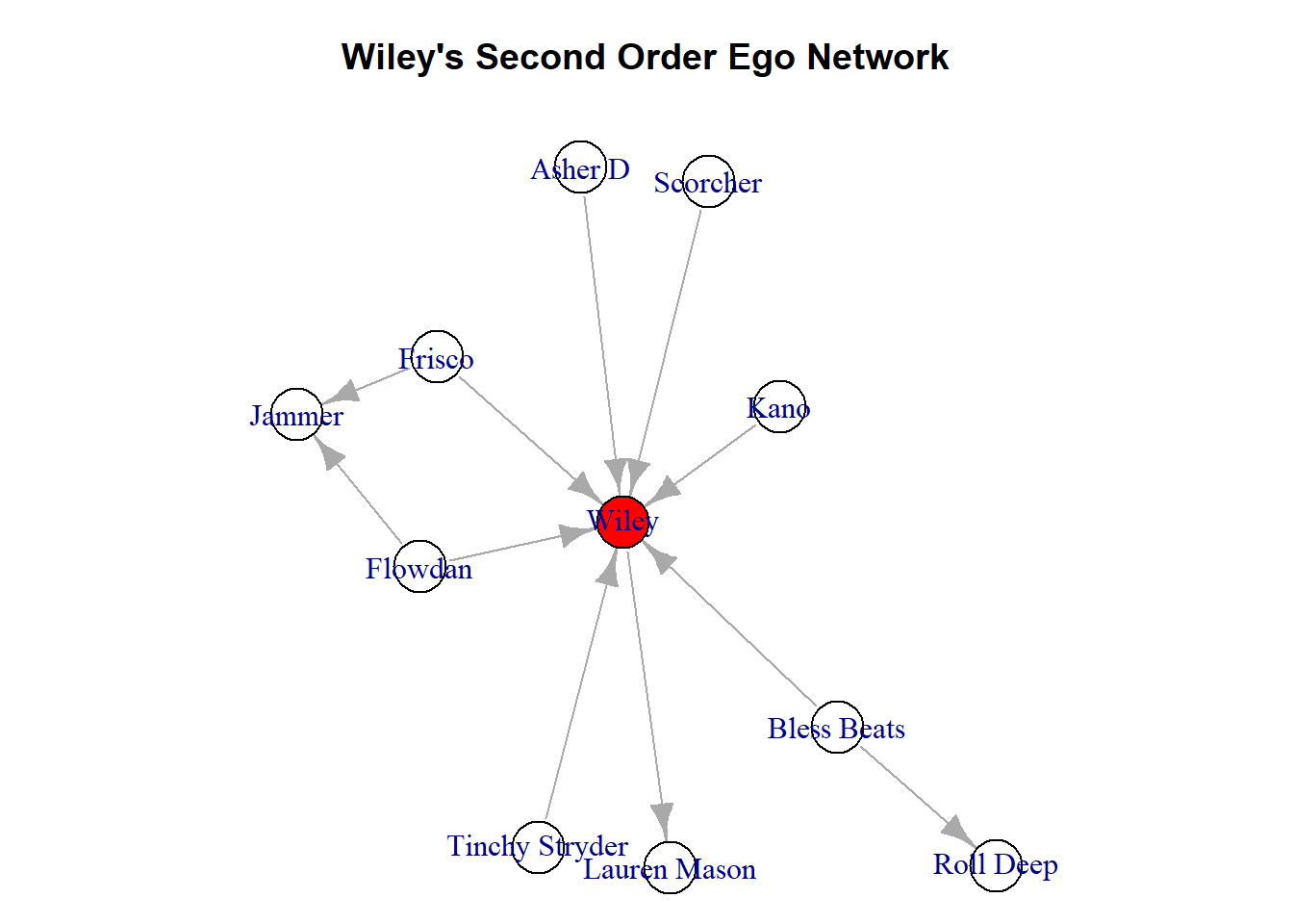
Let’s say there was a person of interest in your network that you specifically want to see. For example, in Grime, the artist called Wiley is somewhat famous for being very well connected to others in the genre. Therefore, we may want to isolate him specifically. You can identify their personal ego network. To do this, you can do the following using the node’s name to single them out. This chunk returns a list of edges connected to Wiley (the name of my node of interest).
E(grime_08_clean)[[.inc('Wiley')]]+ 8/28 edges from 635c771 (vertex names):
tail head tid hid collab_weight
1 Asher D Wiley 1 29 1
2 Scorcher Wiley 4 29 4
3 Bless Beats Wiley 5 29 1
4 Flowdan Wiley 6 29 3
5 Tinchy Stryder Wiley 7 29 2
6 Frisco Wiley 8 29 1
7 Kano Wiley 9 29 1
27 Wiley Lauren Mason 29 39 1Rather than just capturing these, we can also plot these connections. To do so, we return to the make_ego_graph() function and make an object with only Wiley’s ego network. The [[1]] simply tells R to get only the first one in the list that make_ego_graph() creates. In this case, Wiley. Using the “order = 1” option, you are selecting to gather Wiley’s immediate neighbours (known as a first order ego network).
Wiley <- "Wiley"
ego_wiley <- make_ego_graph(grime_08_clean,
                            order = 1,
                            nodes = Wiley)[[1]]

par(mar = c(0,0,0,0))
plot(ego_wiley)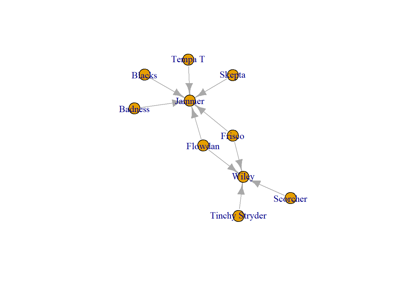
The second order ego network includes the connections of Wiley’s neighbours. This is useful to see whether/how Wiley’s connections are also collaborating. Below we simply change the order to 2. By doing this, we see that Wiley’s collaborators are not working with each other but a few of them are working with others in this network.
second_order_wiley <- make_ego_graph(grime_08_clean,
                                     order = 2,
                                     nodes = Wiley)[[1]]

par(mar = c(0,0,0,0))
plot(second_order_wiley)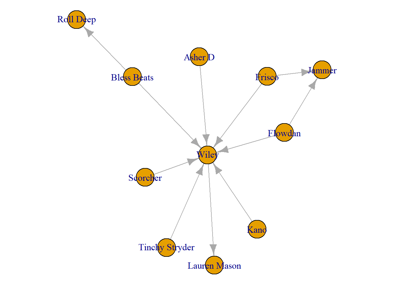
Pro tip: If you are working with ego networks like this, especially when you get passed the first order network (including friends of friends) it is good practice to do something to differentiate the ego from their neighbours. This way, someone who is looking at the graph can clearly identify who is the ego and who are the neighbours. One simple way it to change their colour.
Don’t get too caught up in this code below. We will cover a lot more of this in future chapters. What we do here is create a node characteristic called ‘ego’. What this characteristic does is assign colours to every node in the network. If the name of that node is “Wiley” (our focal node or ego) then the colour is red, otherwise it is white. The next line in the chunk changes the parameters of the plot so we can see it a bit easier. Finally, using the vertex.color option of the plot() function, we change the colour of the visualisation to reflect the red and white that we just added.
V(second_order_wiley)$ego <- ifelse(V(
  second_order_wiley)$name
  %in% c("Wiley"), "red", "white")

par(mar = c(0,0,3,0))

plot(second_order_wiley,
     vertex.color = V(second_order_wiley)$ego,
     main = "Wiley's Second Order Ego Network")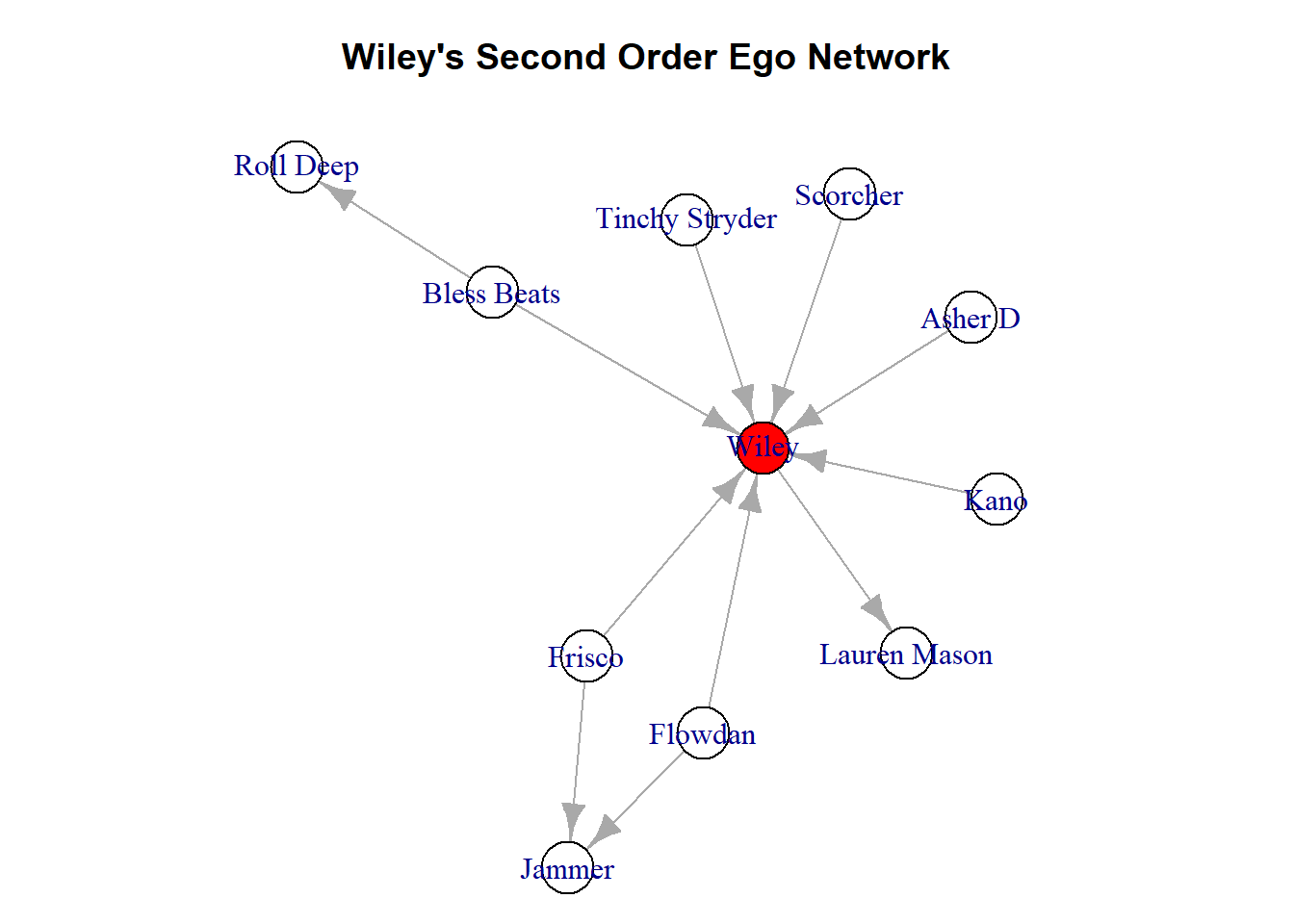
Summary
Here we have discussed another method for transforming network data, taking a subgraph. This is a simple tool that allows you to study a subset of your data. We have covered how to take a specific subset based on the names of particular nodes of interest. Alternatively, we can we can create ego networks for each person in the network or a focal node.
Remember the following:
When taking a subgraph, think about why. Are there specific people you want to study, or maybe you want a network of individuals who share characteristics. Make this explicit in your report/article. This is a subset of your full data so be ready to talk about and justify why you chose to subset it.
Ego graphs and networks lists. This is a tricky data type for new data-users to get used to. Think of Rstudio like a backpack that you store things in. A list can be one of them. The list object that we created is like a segmented container with ego networks in each segment.
Visualise the ego. When making visualisations of ego networks, always differentiate ego from others somehow so it is clear whose network this is.
Great work!!