3  Categorical Data

library(ggplot2)
library(dplyr)
library(gcookbook)

hybrid <- read.csv(file.choose())

3.1 Basic Bar Chart

ggplot(hybrid, aes(x = class)) +
  geom_bar()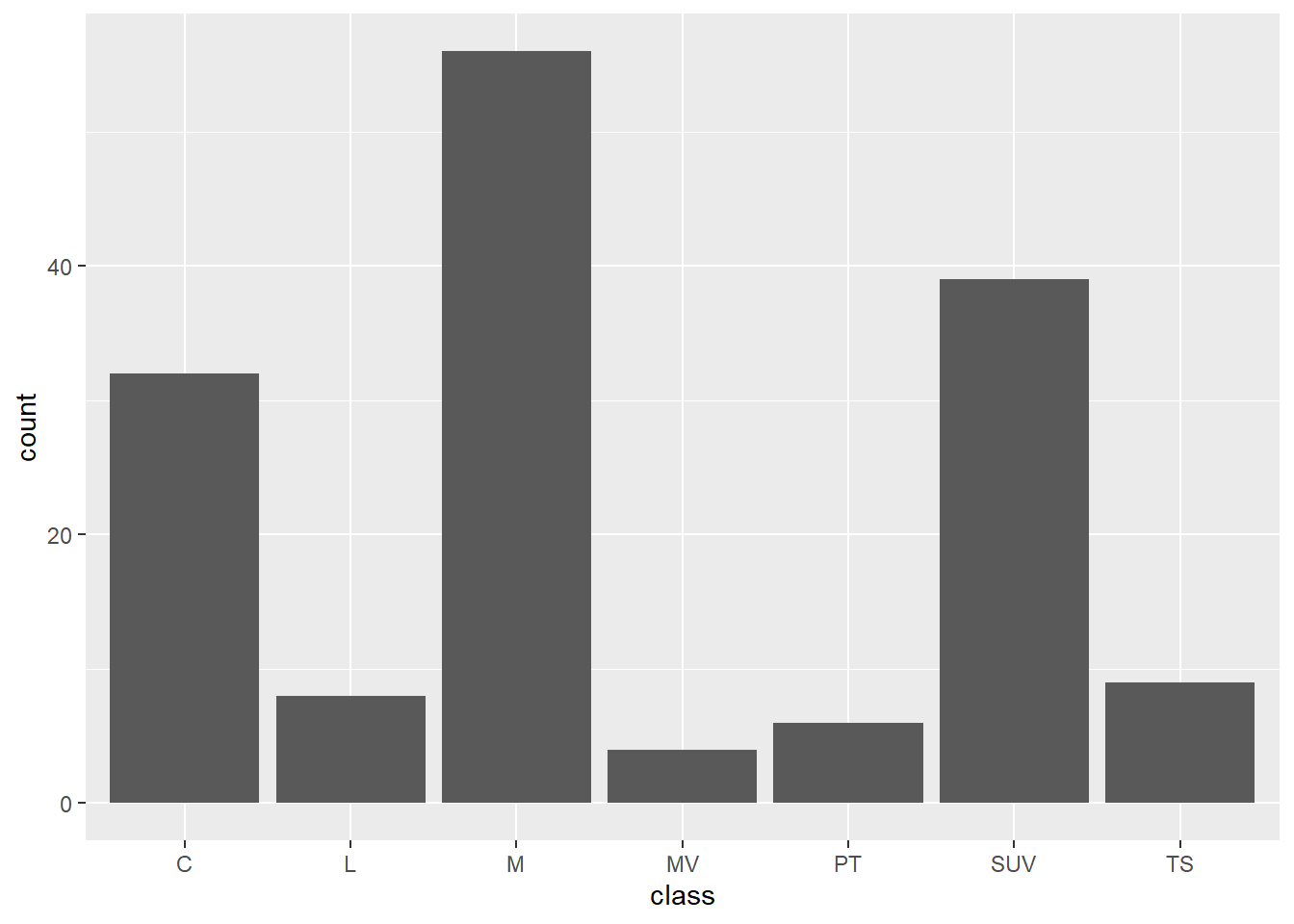

However, this basically serves as a histogram, counting the number of cars in each class type. We may want to so something a little bit more than that. For example, we might want to show the average price of each class of car. to do this, we nee to transform our data a bit. We have mrsp for each car. So, to get the average cost of each class of car, we need to group the data by the class and then get the average cost by that class. Follow the logic of the next chunks of code and look at what the plot tells you.

class_costs <- hybrid %>%
  group_by(class) %>%
  summarise(cost = mean(msrp, na.rm = TRUE)) %>%
  ungroup()

ggplot(class_costs, aes(x = class, y = cost)) +
   geom_col(fill = "steelblue", color = "black") +
  theme_minimal()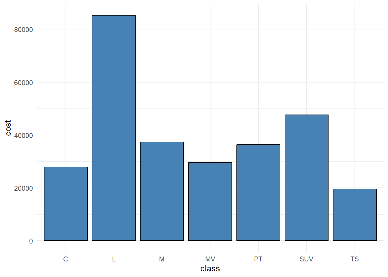

3.2 Intermediate Bar Graphs

Here, we are going to further transform th data to demonstrate some more uses of bar charts. You want to present a bar chart sowing the number of cars in each class by their fuel efficiency.

First, we need to create a categorical variable indicating a a ranking of how fuel efficient the car is. Here, I create three tiers, low (less than 20), medium (20-30) and high (above 30).

hybrid <- hybrid %>%
  mutate(mpg_tier = case_when(
    mpg < 20 ~ "Low (<20)",
    mpg >= 20 & mpg <= 30 ~ "Medium (20–30)",
    mpg > 30 ~ "High (>30)"
  ))

You may want to show the contribution that individual groups make to the total, in this instance, you can use a stacked bar chart. In this case, the stacked bar

ggplot(hybrid, aes(x = class, fill = mpg_tier)) +
  geom_bar()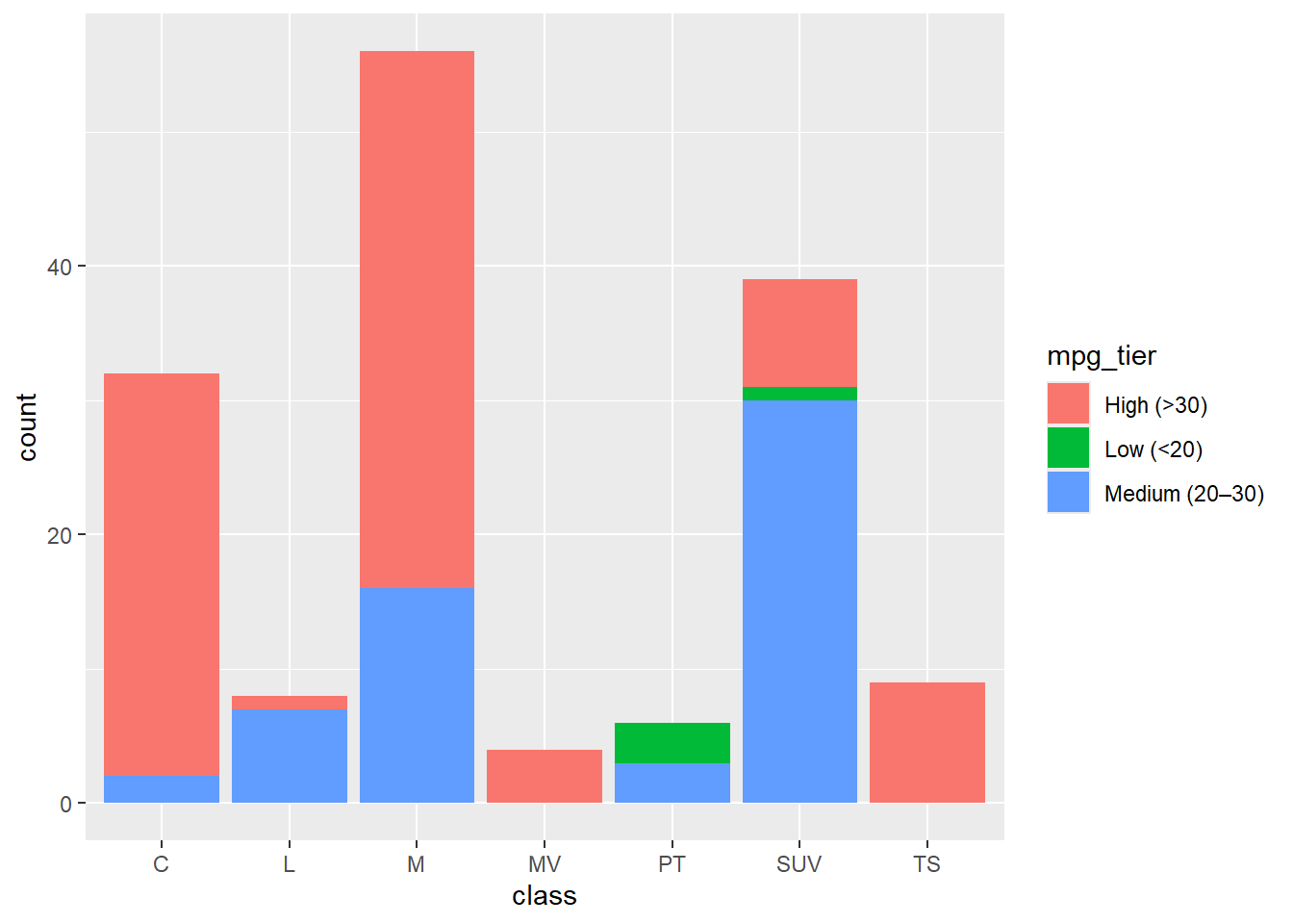 

What types of things do you see here?

This visualiation can be cleaned a little further by adding boundaries around each group. You can also flip the axes to increase readability.

ggplot(hybrid, aes(x = class, fill = mpg_tier)) +
  geom_bar(color = "black") + 
  coord_flip()

Finally, one slight alteration of stacked bar graphs is to scale the y axis to a percentage where 1 = 100% of the total observed at each level of the X axis (note that this total might be different in terms of raw count). This way, each stack of the bar graph represents the proportion of that whole. This is ONLY appropriate if you don’t need to show the count, but care more about the proportion of the total. I.e. the growth in the presence of one category compared to another. This could be missleading since the stacked bars appear to be the same “height” at each category of the X axis. Meanwhile, we know from the above bar graphs that the total (in terms of a count) changes at each category of the X axis.

These are best interpreted when the focus is on relative composition within categories, rather than absolute differences in size. They are particularly useful when comparing how the distribution of subgroups (e.g., MPG tiers) changes across another variable (e.g., car class), while disregarding the total count in each category. However, care should be taken in interpretation: because all bars are scaled to the same height, it can obscure the fact that some groups are much larger than others in absolute terms. If readers misinterpret the chart as representing both proportion and quantity, it can lead to false conclusions.

ggplot(hybrid, aes(x = class, fill = mpg_tier)) +
  geom_bar(position = "fill", colour = "black") +
  coord_flip()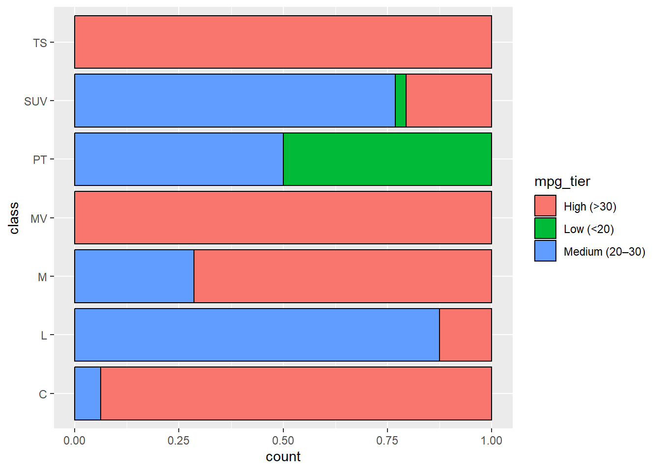

Stacked bar charts are a good tool to have in your toolkit. However, they aren’t always the most intuitive to interpret. Especially if you have more categories than two. In this case, you have three categories. So, if your stacked bar chart is not easy to read, you might decide to place the bars next to each other. This will present three mpg tiers for each class of car.

ggplot(hybrid, aes(x = class, fill = mpg_tier)) +
  geom_bar(position = "dodge", colour = "black")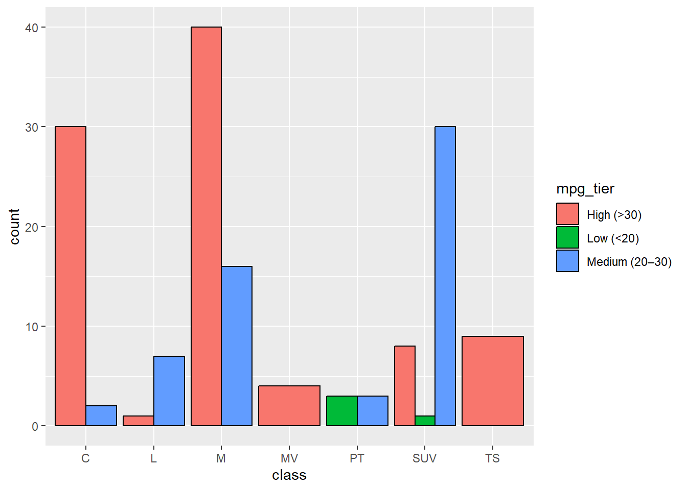

3.3 Pie and Donut Charts

You might be tempted to mock up a quick pie chart when you have categorical data. You can do this in ggplot2. However, don’t. Pie charts are criticised because humans cannot differentiate angles very well. Each segment relies on differentiating from others by their size. If you must make a pie chart, then add the numbers so people can trick themselves that they always knew the segment with 11 is bigger than the segment with 9!

class_counts <- hybrid %>%
  count(class)

ggplot(class_counts, aes(x = "", y = n, fill = class)) +
  geom_col(color = "black") +
  geom_text(aes(label = n), position = position_stack(vjust = 0.5)) +
  coord_polar(theta = "y") +
  theme_void()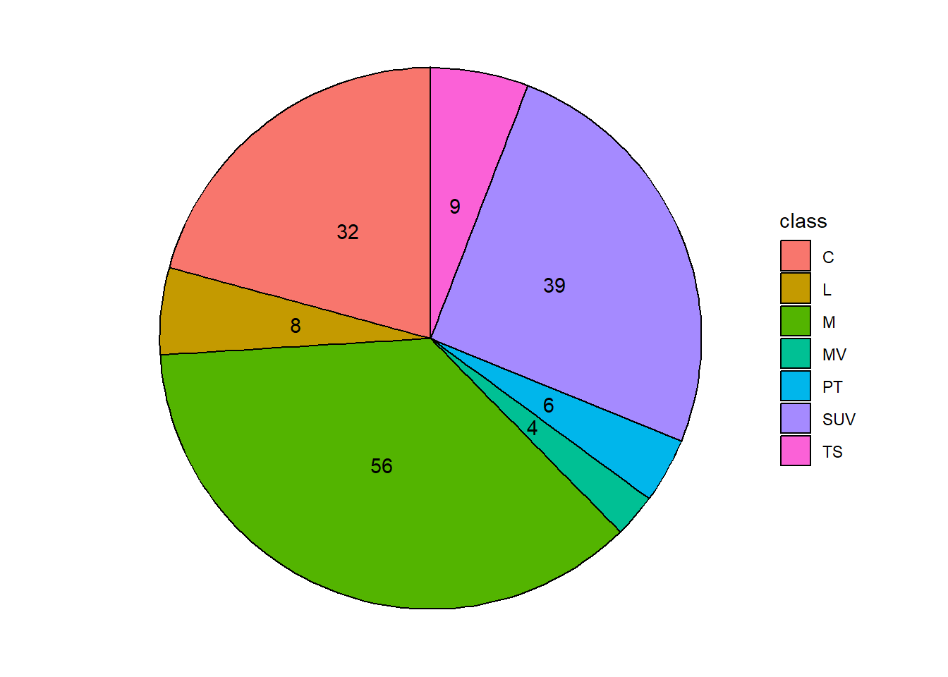

Bar charts are always prefferable. However, if you like the circular vibe consider a donut chart. This is a sort of pie char/bar chart hybrid. Still, not the clearest. To do this, you need to create a variable that demonstrates the hole side (the bigger the number, the larger the hole).

hole <- 5
class_counts <- class_counts %>% 
  mutate(x = hole)

ggplot(class_counts, aes(x = hole, y = n, fill = class)) +
  geom_col(color = "black") +
  coord_polar(theta = "y") +
   geom_text(aes(label = n),
            position = position_stack(vjust = 0.5)) +
  xlim(c(0.2, hole + 0.5)) + 
  theme_void()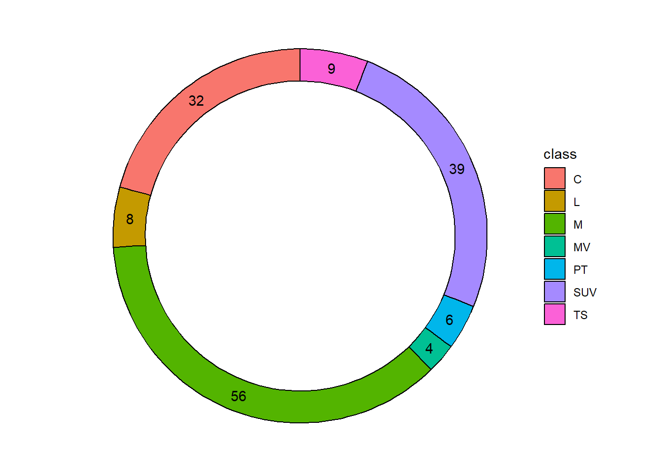

3.4 Activities

From Winston Chang’s R Graphics Cookbook:

• 3.5 - Negative and Positive Values